(Note: this is a reduced-jargon/increased fun version of a paper published on Arxiv here: https://arxiv.org/abs/2509.18103. Thanks go to my co-authors: Michael Joedhitya, Adith Ramdas, Surender Suresh Kumar, Adarsh Singh Chauhan, Akira Rafhael, Wang Mingshu and Nordine Lotfi.)
Is maths invented or discovered?
Most non-mathematicians will say it is discovered. Here is one thing, and there is another thing, and now we have two things: tada. On the other hand, there is a small subset of theorists (such as Leopold Kronecker) who argue that while much of it is not true, it is nevertheless often useful: Negative numbers do not exist in nature, but they make the sums we need to parse nature a lot easier. There’s no such thing as the square root of a negative number but pretending there is provides us with a handy drawer in which to store multi-dimensional values and thus imaginary numbers were born.
This is the line taken by the publishers of the Nature journals, who, when they are asked why there is no Nature Mathematics, patiently explain that it is because maths is not a science, being a matter of logic rather than empirical investigation.
The problem with this clear division comes when the numbers start doing things that they weren’t designed to do, or - conversely - don’t do what you would expect them to: when deterministic processes yield seemingly random outputs, or when phenomena predicted by maths coincidentally pop up in physics (or vice versa). These cases are interesting because they seem to imply that both maths and physics are something like images projected onto the surface of a unified underlying structure - the manifold of the possible[1]. Invisible itself, it is the rule set that determines the possible rule sets, meaning that we can only guess at its shape by looking at the ways in which observable rules converge or diverge.
If you’re a statistician this is great insofar as that it drags numbers back into the empirical world, putting them within reach of probabilistic analysis tools such as AI models. If they are simply a formal language built for expressing logic operations precisely, there’s not a lot we can do with them. If they’re shadows on the wall of nature, it’s perfectly reasonable to treat them as a dataset like any other, and while models aren’t necessarily great at solving equations or proving identities, they’re superlative when it comes to spotting patterns in the results once they’ve been found[2].
One example of this would be the patterns in prime numbers, which have been tantalising mathematicians for centuries. Prime numbers aren’t predictable but do crop up at a pretty predictable rate.
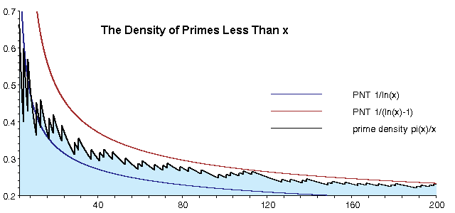
Give me a number and I can tell you roughly how many primes there will be in the vicinity, but not easily predict with any reliability whether the next one will be two, three, four or five numbers away. That’s not all, however, there are various ideas in number theory that suggest that not only do prime numbers become less frequent the further you go, they also settle into more predictable patterns, with small differences having big ripple effects near zero that gradually even out as you head further out. The theories suggest that this is not a product of true order, but rather because their irregularities obey reliable statistical laws that only become apparent at very high numbers. Unlike physical systems, primes don’t “evolve” in time, but as you move along the number line, you see a statistical equilibrium emerge between order (the global density law, equidistribution in progressions) and disorder (random-looking gaps).
We wanted to investigate this using AI models, not with the aim of predicting next primes accurately, but to try to isolate the underlying patterns and non-linearities that create this infuriating quasi-order.
To do this we started by arranging the numbers in an Ulam spiral format - a spiral representation in which primes are coded in one colour and composites another.
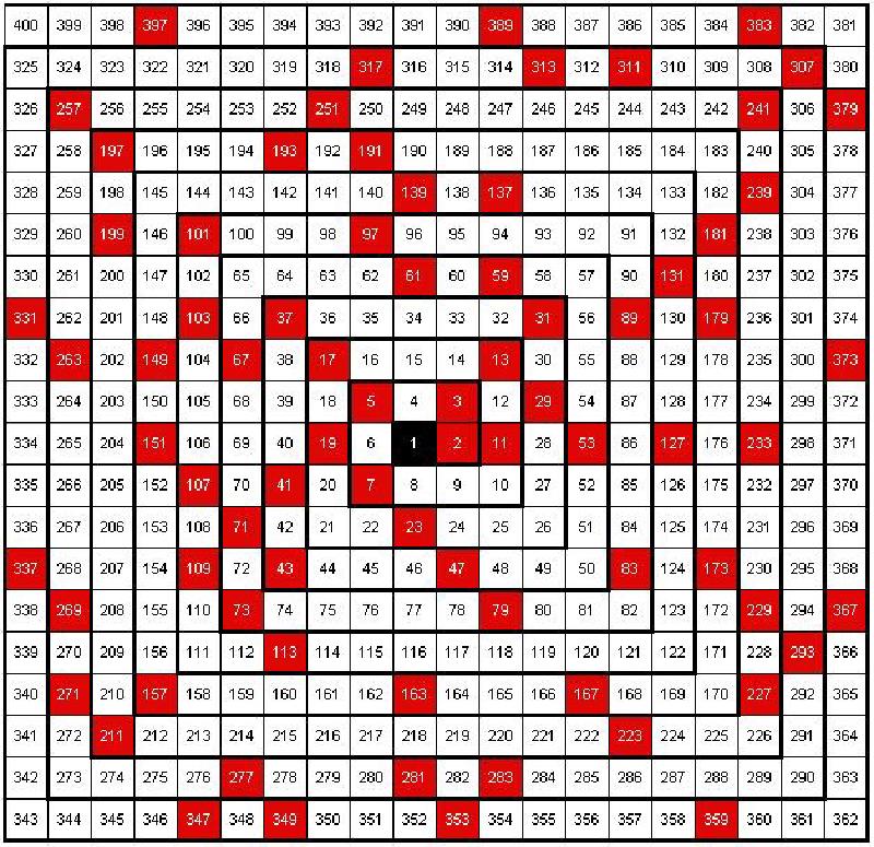
It produces intriguing suggestions of order to even a casual human observer:
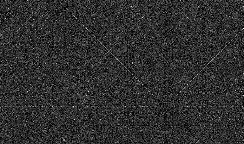
If we run a fast Fourrier transform on the image to give us a broad idea of the noise-to-signal ratio, it’s even more impressive, producing a beautifully ordered fractal snowflake that hints seductively at multiple overlapping signals/rulesets in the original that would be a great explanation for why accurate predictions are so hard to make. (If you want a basic guide to interpreting these patterns, there’s an introduction to the Fourier transform.)
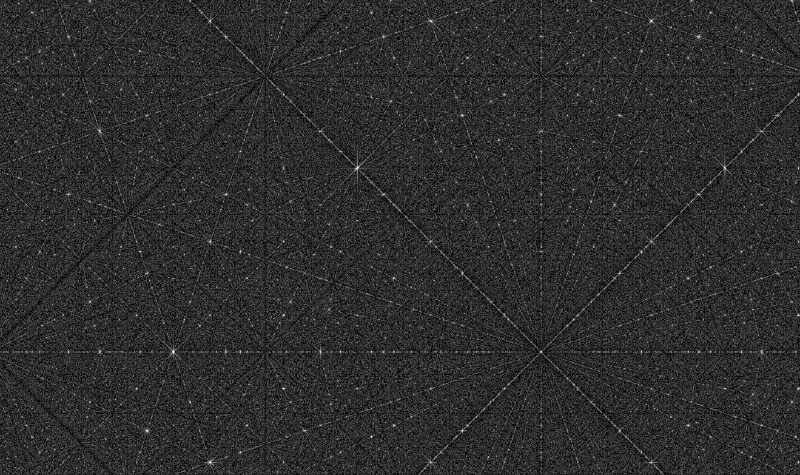
This Ulam spiral format is definitely the layout in which humans find patterns easiest to identify, so the team reasoned that an in-painting model - that is an AI that tries to guess what is in a masked out part of an image when given the remainder - would probably be even better.
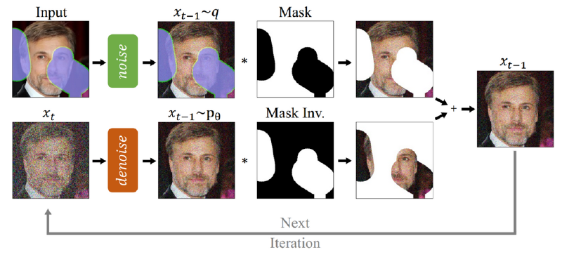
To train our model we generated black-and-white Ulam spiral images en coding consecutive integer sets:
• n < 25,010,001 (5001×5001 pixels),
• 25,010,001 ≤ n < 50,027,329 (7073×7073 pixels),
• 50,027,329 ≤ n < 100,020,001 (10,001×10,001 pixels),
• 100,020,001 ≤ n < 200,024,449 (14,143×14,143 pixels),
• 200,024,449 ≤ n < 300,017,041 (17,321×17,321 pixels).
• 300,020,041 ≤ n < 400,040,001 (20,001×20,001 pixels), and
• 400,040,001 ≤ n < 500,014,321 (22,361×22,361 pixels).
Each image was chopped into 350 non-overlapping blocks of 256×25 pixels each (this is a reasonable size to favour the learning of both local and global patterns. Each set of blocks was divided into training (300) and validation (50) sets.
We used these to train a two-dimensional U-Net with a ResNet-34 encoder pre-initialized on ImageNet. It’s a pretty basic model architecture but the goal here was easy replication rather than high performance, given that our broader aim was to study the learnability of the patterns rather than to achieve the best possible predictions. In this case the same basic model model was trained on each spiral and subsequently evaluated across all test sets - so the 25m model was tested on the 25m test set, but also on the 50m, 100m, 200m etc. sets. Comparative performance was used as a proxy for the learnability of prime patterns within each numerical range. To confirm broad trends and minimise chaotic fluctuations in output at the individual model level the process was repeated three times and an average taken. To account for the limited dataset size, we employed resampling with n = 10,000 replicates and computed confidence intervals for all reported metrics. Likewise, to control for the effects arising from the differing proportion of primes in lower and higher areas of the spiral, we checked the threshold binarisation model against a top-k binarisation model[3].
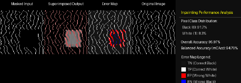
For each test, the model produced five outputs: (i) the masked input, (ii) the in-painting reconstruction, (iii) the pixel-wise error map, (iv) the ground-truth image, and (v) summary statistics.
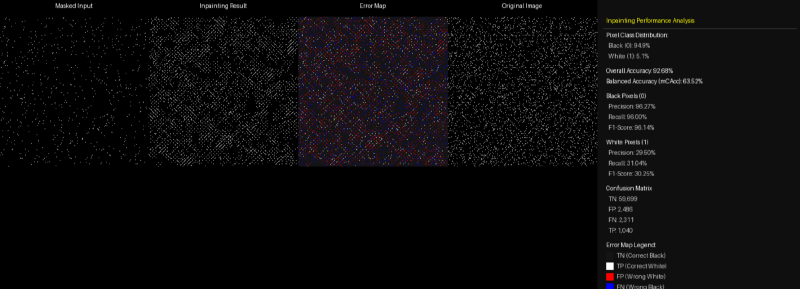
However, if one attempts to maximise for raw accuracy on such a task a problem immediately appears. Because any given image is around 5-6% white pixels and 94-95% black, a model that simply predicts nothing but black pixels will already be scoring almost 100% accuracy, and will most likely settle for this, since any attempt to do better will certainly result in worse scores, at least initially. In place of this, we focused on maximising for mean class accuracy - i.e. a metric that would overweight the white score to make seem as if white pixels made up half of the total, rather than just a tiny fraction. You can see the dramatic difference this makes in the tables below. Here the columns show the accuracy that a model trained around a particular region of the spiral (25m, 50m etc.) achieved when attempting to in-paint images taken from both the same and different regions (red = more accurate).


In other words, the model looks like it’s better at predicting primes at low numbers, and composites at high numbers. We can actually go deeper and check this via the precision (what proportion of pixels predicted to be [colour] were actually [colour]), recall (what proportion [colour] pixels were predicted to be [colour]) and and F1 (precision times recall over precision plus recall times two) stats.
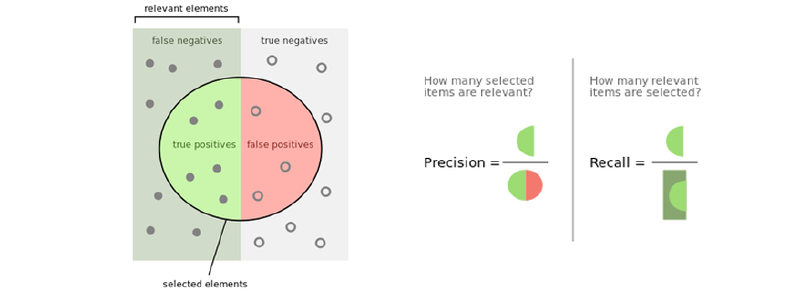
Thus decomposed, the intuition is confirmed. The model starts out predicting primes, but shifts towards predicting composites, identifying primes only by elimination.
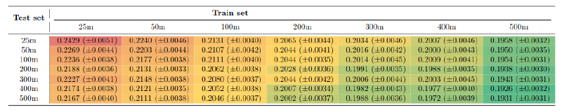
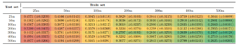
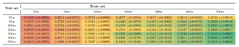
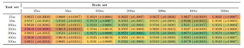
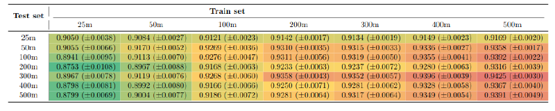
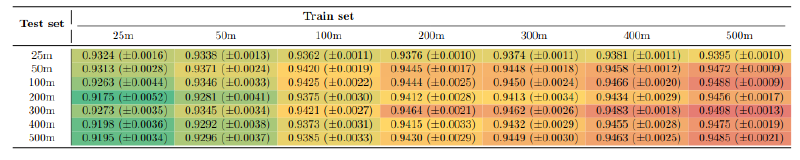
But there’s something else going on here too. There’s a clear step-change between the 25m set and the others. This was also visible in the training records
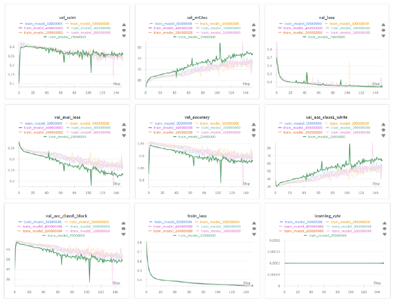
But there’s something else going on here. Given the known prime density at each region, it is possible to work out what scores a model would achieve if it knew the rough proportion of black-to-white pixels would be present in a given region, but had no knowledge of pixel patterns.
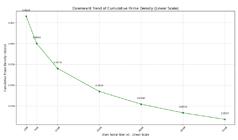

Firstly, and most obviously, it is worth noting that while a model that simply guessed based on white:black ratios in a given region without learning patterns would achieve similar black and overall scores to the model we describe above, it would score significantly lower on white metrics, suggesting that our model shows a degree of pattern-awareness.
However, it also becomes possible to compare the rates at which prime prevalence and prime pattern learnability diminish.
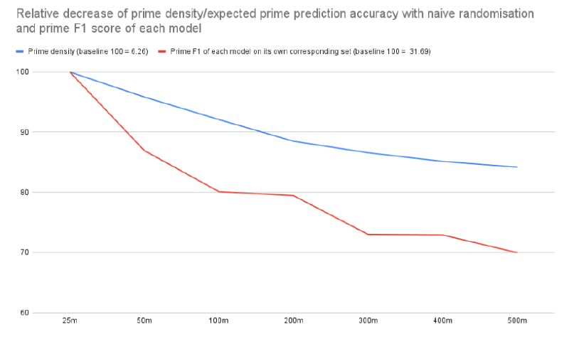
When we do this we observe that the learnability of the prime patterns diminishes much faster than the prime density, with the biggest drop being between 25m and 50m.
So what should we conclude from this?
- Primality is not simply an absence of compositionality. It’s something else.
If this were the case one would expect the prime and composite F1 tables to be more or less identical. Instead they are mirror images of one another. the model is not simply learning white vs. non-white or black vs. non-black, it perceives white and black as separate categories with different sets of characteristics. This would fit with the idea that each is the product of multiple overlapping deterministic filters.
- The importance of prime patterns declines faster than you’d expect.
When we started on this, we were prepared for the possibility that the learnable quasi-order in the primes may actually diminish so slowly that it simply would not be detectable at the scales to which our computing power grants us easy access - i.e. they would only be visible in spiral generations that would require unfeasible amounts of compute power to generate. This is not the case - in fact a major part of the drop happens below 50m.
This opens up a whole lot of fun cryptographic applications, whether defensive (improving the model to use as pre-filter when searching for n n-bit primes, spotting areas of strong and weak primes based on semi-prime spiral data) or offensive (training a discriminator model on primes generated by an existing algorithm vs. reference primes to spot non-uniformities). However, the idea of machine learnability as a measure of order also has potential when it comes to exploring Riemann/Chowla-related processes that are conjectured to behave like random coin-flips. If an appropriate model achieves anything better than 50% accuracy it is potential evidence of order - not necessarily disproving any of the relevant conjectures but providing nuance. So, for example, Chowla says correlations like λ(n)λ(n+1) should average to 0 - if the model consistently finds signal, it could be seeing slow convergence or hidden local structure. Likewise, Riemann implies specific bounds on prime irregularities; if a model beats random at predicting primes in certain windows, this helps to refine the bounds and identify specific fluctuations.
However, the same basic model also does well in entirely unrelated areas - even better in some cases. Here it is crushing state-of-the-art validation metrics in geological fault prediction:
In each case, however, the most interesting fact is not that this is possible but that it opens up the possibility of isolating features that contribute to the overall result. We didn’t do it here (because, well, it’s time-consuming and fiddly and we have day jobs), but it’s perfectly possible to work out how certain the model is about specific pixels and identify the commonalities, thereby working back to find the specific sieves that the AI thinks are most important. Likewise, by layering geological datasets and feeding them into a model we can identify the precise features that are most important in locating mineral deposits. In each case the AI isn’t necessarily finding the answer, but it’s telling us why we should expect to find the answer in a given place.
[1] One neat example of this would be string theory. Experience has showed us that when you break things down into their constituent parts you get a series of ever smaller particles, so you might expect that if you keep going you’ll eventually reach a dimensionless point-particle of pure essence. The problem with this is that if we insert it into our current load-bearing maths stack, it would produce a universe that was essentially a singularity at every point. We can’t change the maths without breaking other things, so the fundamental particles must be some other shape. Fortunately, if you simply assume that they’re a one dimensional string, not only do the equations work out and produce a reasonable universe, they also imply the existence of gravitons, which was implicitly confirmed by the observation of gravity waves in 2015. In this case the mathematical rules were established first, but turned out to be a projection of other fundamental physical properties of the universe.
[2] Deepmind in particular has been going hard on this angle lately, having hired Javier Gómez Serrano - probably the primary specialist on Navier-Stokes out there - with the specific goal of cracking a Millennium prize problem using AI. They haven’t cracked it yet, but they just published some neat unstable singularities.
[3] Where the base model assigns a given pixel as white if the likelihood of it being white passes 50%, the top-k model automatically assigns the top xx% of pixels white. This allows us to control for the effect of the different proportion of primes at different regions of the spiral. The full results can be found in the original paper.