Ever since humanity began interacting with LLMs, we also began co-creating a new vocabulary to describe it. Sure there’s “slop” and “4oid” but also “load-bearing”, “metaconcept” and even possibly ideas like “test-time adaptation”, whose adoption seems to have been heavily influenced by conversations between developers and their LLMs.
We wanted to track interest in different AI related concepts over time, but not just this. We wanted to spot the semantic basins of attraction that seemed most active and fertile when it comes to linguistic invention. What ideas are tech people circling around that aren’t yet named, and what do the LLMs want to call them.
That was the genesis of the Reports From The Future project. This mini-site features:
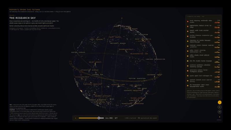
A six-month mapping of Arxiv paper topics, with redder clusters being hotter at any given moment.
Plate I — The Research Sky A Three-month lexical mapping of topics being discussed on X.com, HuggingFace Blogs, LessWrong and other trend-setting AI venues, with a slider allowing users to isolate weekly snapshots. This focuses on the technology, isolating particular tech clusters that are being discussed intensively in a given week. As before, redder clusters are hotter.
Plate II — The Attention Sky The same thing, but with clusters focusing not on lexical but semantic proximity. Clusters that share a latent space but use diffuse vocabulary (gold) imply a concept being born, when semantic and lexical similarity are both high (red) that’s an established trend, and when the same terms are being used in different contexts (purple) that’s a sign that we’re moving into buzzword territory. For maximum compression we asked a panel of four LLMs (Gemini, Grok, Haiku and 4o mini) to describe what features defined each cluster, and had Fable extract the core metaconcept from these descriptions (details bottom left).
Plate III — The Emergent Sky
For anyone who wants to get a deeper understanding of the algorithm, we include a detailed description below.
How the three star maps are made
Notes on the method behind the three plates in Reports from the future. Every star is one source document: a paper, a post, a tweet.
The shared pipeline
All three plates come from the same three steps. What differs between them is how constellations get named, which ones get named at all, and what the colour encodes.
1. Each document becomes a vector
Title and text go to an embedding model (text-embedding-3-small), which returns a 1,536-dimensional vector. Documents about the same subject land near each other in that space even when they share no vocabulary: “the model overfits” and “the network memorised the dataset” are neighbours there, with no words in common.
2. UMAP reduces the vectors to something drawable
UMAP compresses the cloud while preserving local neighbourhoods. The settings are the same throughout: 15 neighbours, min_dist 0.05, cosine metric.
The fit runs once over the whole corpus and is then frozen. UMAP is unstable under changes to its input, and re-fitting on a slightly different document set can rotate, mirror or rearrange the entire map. A per-week projection would scramble the sky every week and make growth indistinguishable from movement. With the projection frozen, a document’s coordinates never change and the slider only alters which stars are lit.
3. HDBSCAN finds the dense regions
HDBSCAN scans the reduced cloud for regions of high point density. Each one becomes a constellation. Points in no dense region are labelled noise and drawn as dust, so a document that sits alone is reported as sitting alone rather than assigned to whichever group is nearest. The minimum size a region must reach is set per plate, scaled to the window being clustered.
The plates do not all cluster the space they draw
Plate I fits UMAP to three dimensions and clusters those coordinates.
Plates II and III do not. Their clustering runs on a two-dimensional UMAP fit, while the sphere is drawn from a separate three-dimensional fit of the same embeddings. The two fits are independent. A constellation can therefore be tight in the space that produced it and still look scattered on the sphere. That is a property of the projection rather than a fault in the rendering.
Names, colours and sliders are all interpretation layered on top of these steps.
Plate I — The Research Sky
Corpus. arXiv papers in cs.AI, cs.LG and stat.ML
Constellations. Minimum cluster size 100, set high because the corpus is large. That yields 105 constellations, and every one of them is drawn. 35% of papers fall outside any cluster and become dust.
What ships. Clustering runs over all sources and caption says how many were left out. Every star is a real paper; not every paper is a star.
Names. TF-IDF only, no model calls. TF-IDF scores terms that are frequent inside a cluster and rare across the corpus, which gives names of the form segmentation · medical · clinical · mri · image.
Colour: publishing rate, not paper count
Colouring each month by its total distorts both ends of the window. i.e. February starts on the 4th, and the last month holds papers for three days because that is where the export stopped. On totals August reads as near-empty, at 6% of the May peak. That number describes when counting stopped, not what was published.
Each month is therefore divided by the days of it the window actually covers. Calendar days alone are not enough: a short span carries an unrepresentative mix of weekdays, and arXiv publishes far less at the weekend. Two of August’s three days are a weekend. The divisor is in weekday-equivalent days, where each observed day counts as its own weekday’s share of an average day. February gets 25.0 days rather than 25, and August gets 2.4 rather than 3.
The correction changes what the plate says. August moves from 6% of the May peak to about 70%, which takes it from last of the seven months to third. And February and March, 22% apart on totals, land within 3% of each other on rate. The gap between them was February’s three missing days at the start of the window.
One absolute scale spans all months, running white through yellow to red.
Slider. The slider moves a light rather than revealing content. Every month’s papers are present as grey dust at every stop and only the selected month is lit, so the shape of the corpus stays constant across stops. Focusing a constellation shows its full extent across the whole window, with the selected month brightest.
Plate II — The Attention Sky
Corpus. HuggingFace Papers, X, Hacker News, LessWrong, the Alignment Forum, and a few blogs.
Constellations. HDBSCAN runs twice over the same projection on different subsets: once over a rolling 91-day background at minimum cluster size 15, and once over each week alone at minimum cluster size 8. The two thresholds differ because the background is roughly twelve times the size of a week, so a single value cannot mean the same thing for both.
The slider steps through the weekly runs, and every constellation they find is drawn: 209 across the eleven weeks, between 13 and 26 in any given week. The background run is not drawn. What the background supplies is the projection and the surrounding documents, which appear as dust and keep the sky from emptying out around each week.
Names. TF-IDF, shown raw. These are the terms the discourse itself uses, and a name that reads badly is information about a cluster whose vocabulary has not settled.
Colour. Cluster size, log-scaled and rescaled inside each week: that week’s smallest constellation white, its largest red.
Rescaling per week costs something. Cluster sizes are long-tailed, and a single absolute scale across the whole window painted one constellation red and left everything else white. Per-week rescaling makes every frame readable, but colour then ranks a week against itself rather than against the other weeks.
Plate III — The Emergent Sky
Corpus and constellations. The same run as Plate II: same weeks, same sphere, same clusters, verified row for row at build time. What differs is how constellations are named, and which ones are named at all.
The target is a specific phenomenon: an idea in circulation before it has a name.
The name gap
Two scores are computed for each weekly constellation.
Lexical coherence is the mean pairwise cosine similarity between the documents’ TF-IDF vectors. It measures shared words.
Semantic coherence is the same statistic over the embeddings from step 1. It measures shared meaning.
Each score is converted to a percentile rank among that week’s constellations:
name gap = semantic rank − lexical rankRanks are used instead of the raw scores because the two are not comparable in magnitude. Embedding similarities run far higher than TF-IDF similarities for essentially every group, so subtracting them directly gives a positive number almost everywhere and separates nothing. Ranking first removes the offset and leaves each constellation’s relative position on the two measures.
A large positive gap means strong agreement on meaning and weak agreement on vocabulary. The documents circle one subject in different words because no shared term for it exists yet.
A large negative gap is the mirror case: strong agreement on words, weak agreement on meaning. One term applied to several different things.
Which constellations get named
Both scores are percentile ranks, so the gaps sum to zero. Every week therefore contains a most-emergent and a most-stretched constellation whether or not either is remarkable. The two ends are selected differently as a result.
On the emerging side, constellations with a positive gap are ranked and the top ones go for naming.
On the buzzword side there is a floor. A constellation qualifies only if its gap falls below −0.3, not merely by ranking last in its week, and at most a few per week are taken. The floor sits at −0.3 rather than −0.5 because at −0.5 one of the eleven weeks has no candidate at all, while at −0.3 every week has at least one and the average is 2.6.
The naming chain
Selected constellations pass through three stages, all routed through OpenRouter.
Four models compress independently. gpt-4o-mini, grok-4.5, claude-haiku-4.5 and gemini-2.5-flash each receive the same documents and separately describe, in one paragraph, what they have in common. A single model’s description reflects that model’s habits. Where four independent descriptions converge, the convergence is more likely to come from the documents.
Claude Fable 5 synthesises. The four descriptions go to one model with a different task: to name the underlying attractor they all gesture at without stating, rather than to summarise them. The instruction is to name it the way a physicist names a phenomenon, specific and conceptually loaded, with no generic AI framing.
Claude Haiku 4.5 distils. The synthesis is compressed to a short noun phrase for the constellation key: Acephalic competence, Behavior underdetermines cognition, Capability ascription decoherence.
Haiku appears twice, once as a member of the compression panel and again as the distiller. The two calls see different inputs and do different jobs.
Inverted prompts at the buzzword end
The two bands cannot share a prompt. The emerging prompt tells the panel that a shared referent exists and asks it to be identified. Handed a buzzword cluster, the models oblige, fluently, and invent the unity that the negative gap is evidence against.
Buzzword clusters get an inverted prompt pair instead. It asks what the shared term is being made to stand for and which distinct senses it now carries, with an explicit instruction not to construct a unifying concept and to say plainly when no single referent exists.
The outputs differ in kind. Two buzzword syntheses, from weeks 5 and 10:
“Claude” is a given name mid-genericide: once a person, then a product, now sliding toward a common noun meaning “whatever an AI wrote.”
“Claude” has stopped naming a model and become a metonym for the whole stack around it — one word standing in, by turns, for the LLM, a pricing tier (“Claude (max)”), a coding agent (“Claude Code”), a running process (“keeps your Claude session warm”), and even the legal liability of its maker (the Anthropic settlement “for training Claude”).
Neither names a concept. Both describe a term coming apart, which is what a negative gap indicates.
Colour. The name gap itself, as a continuous ramp: indigo #4338ca at −1.0, purple #9333ea at −0.5, red #dc2626 at 0.0, orange #ff9628 at +0.5, pale gold #ffe082 at +1.0. The band words in the key are a coarser reading of the same number, with cutoffs at ±0.33.
Slider. Each week is clustered and named on its own, so the slider steps between frames rather than accumulating a reveal. Cluster identities do not persist from one week to the next, and a theme recurring under a different name is expected. That drift is what a map of unsettled vocabulary is there to record.